Similar to SG's suggestion, but including highlighting for both MAX and MIN values in column B, and doing a single calculation of the MAX value and on the MIN value in that column:
 Formula in C2: MAX(B)
Formula in C3: MIN(B)
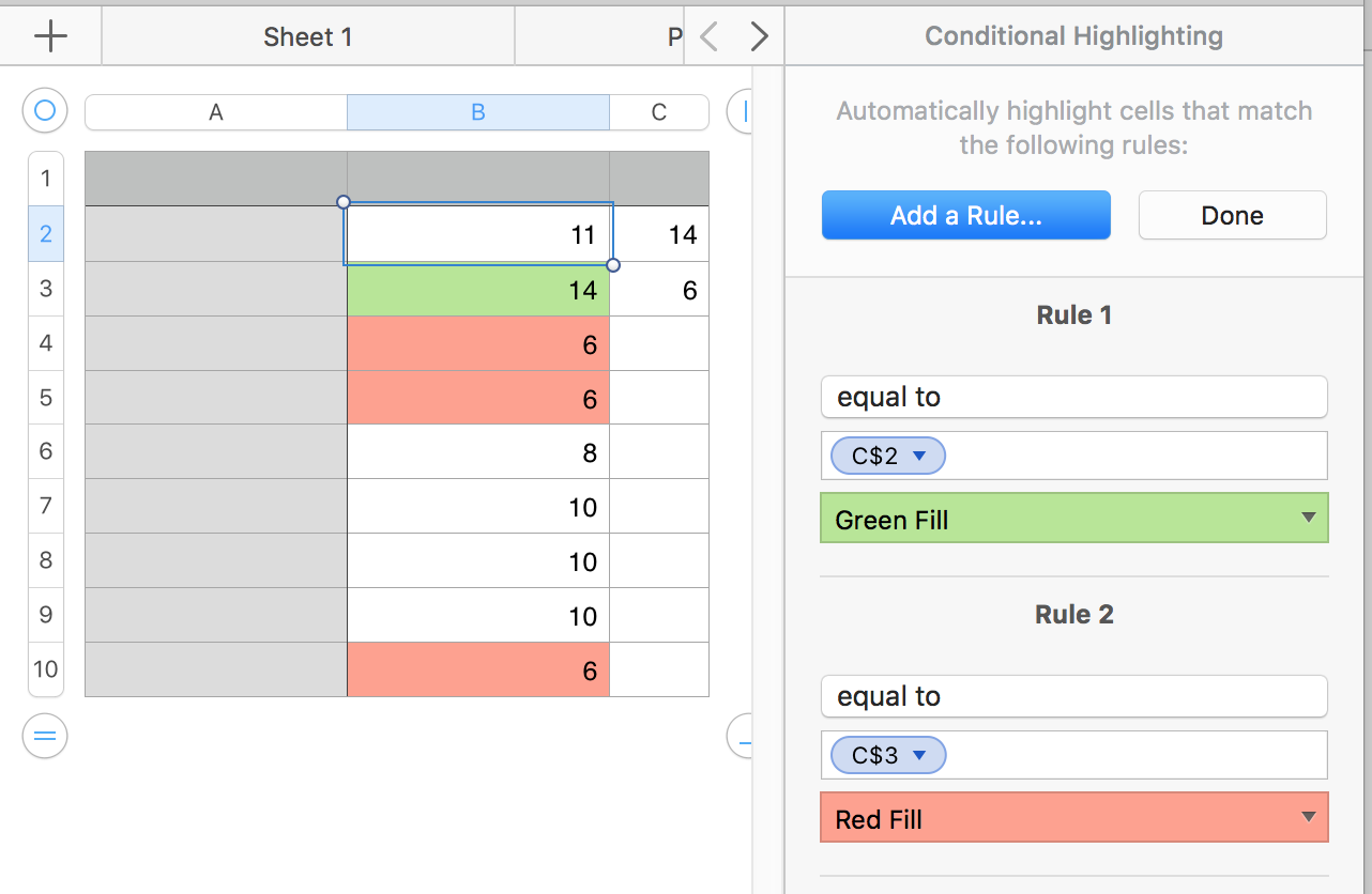
Enter the two formulas in their respective cells, then click on cell B2 to select it, click the Conditional Highlighting button at the bottom of the Cell section of the Format Inspector and construct the two rules shown.
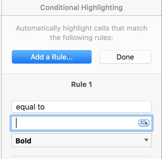
After clicking 'Number' and 'equal to', click the icon at the right end of the entry br (see image below), then click the cell containing the Max formula (C2 in the example).
With the C2 token in the box, click the triangle to the right of C2 and choose Preserve Row to insert the $ operator.
Then choose the highlighting you want for the MAX value.
Click Add a Rule again and repeat the steps above for the MIN highlighting rule.
After entering both rules, Click Done, then:
Select B2 and all of the cells to be governed by these conditional highlighting rules.
In the inspector, choose Combine Rules to apply these two rules to all of the selected cells.
Regards,
Barry