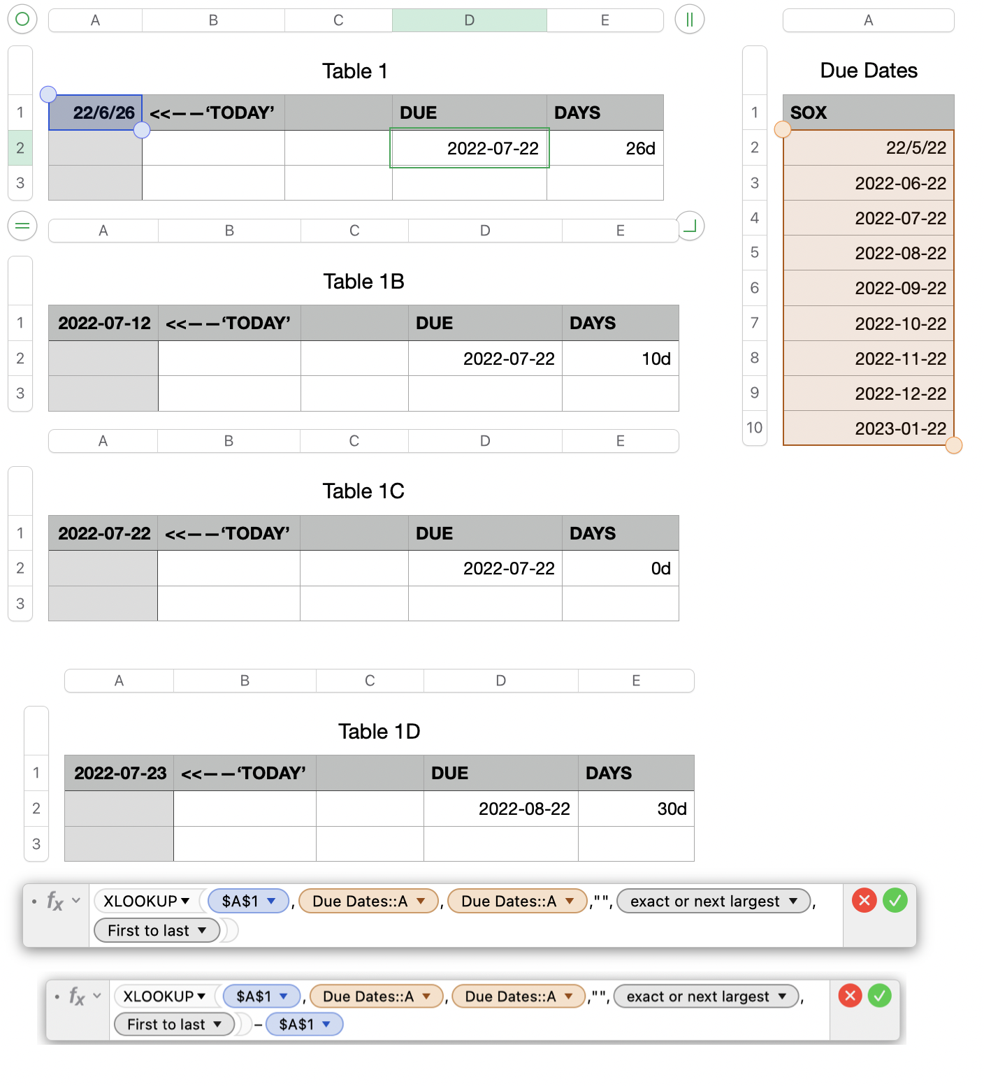
Here's one way, using an auxiliary table to contain the 'fixed day of month' due dates.

See note below before entering the bottom formula above in E2.
It can be significantly simplified!!
Table 1, Table 1B, Table 1C and Table 1D are images of the same table as it appears on four different dates.
In practice, cell A1 would contain the TODAY() function, which returns the current Date. In the example, it contains the four dates shown, uses to show the results in D2 and E2 on each of those dates.
The smaller table contains an entered date in A2, and the list of future due dates at one month intervals in the rows below that. The list was created by entering the first two dates directly to establish the interval between them, then selecting both cells and dragging the Fill Control (small yellow filled circle) that appears on the bottom boundary of cell A3 and dragging down the column as far as needed. An alternate would be to use the EDATE function to generate the rest of the list from the first entry in A2.The two formulas shown below Table 1D. The upper one uses XLOOKUP to search column A of Due Dates to find the first due date that is on or after the date ('TODAY') in A1 of Table 1.
The second formula is exactly the same as the one just described, and exists only because it was in the first cell I placed a formula in. It differs from the formula in the same row of column D only in subtracting 'TODAY' from the result calculated by that formula.
Rather that doing that calculation twice, delete everything from the longer formula except the -$A$1. Replace the deleted part with s direct reference to cell D2, where that calculation has already been done,
giving this formula for E2: 
Regards,
Barry