First thing is to put a date on every line that has a time. You can continue with it as two separate columns but it might be less hassle to use one column that has the date and time in it like 07/07/25 6:36AM. If you type just the time, it will be given today's date without having to type it. Once all data rows have a date, you can use SUMIFS to sum them by month in your other table (see below).
If you used the first table only for data and there were no "total" rows, you could make a pivot table instead of using SUMIIFS. Maybe you can do it with the "total" rows there. SGIII might help with this. I don't do pivot tables very often but it would save you from a whole lot of formulas.
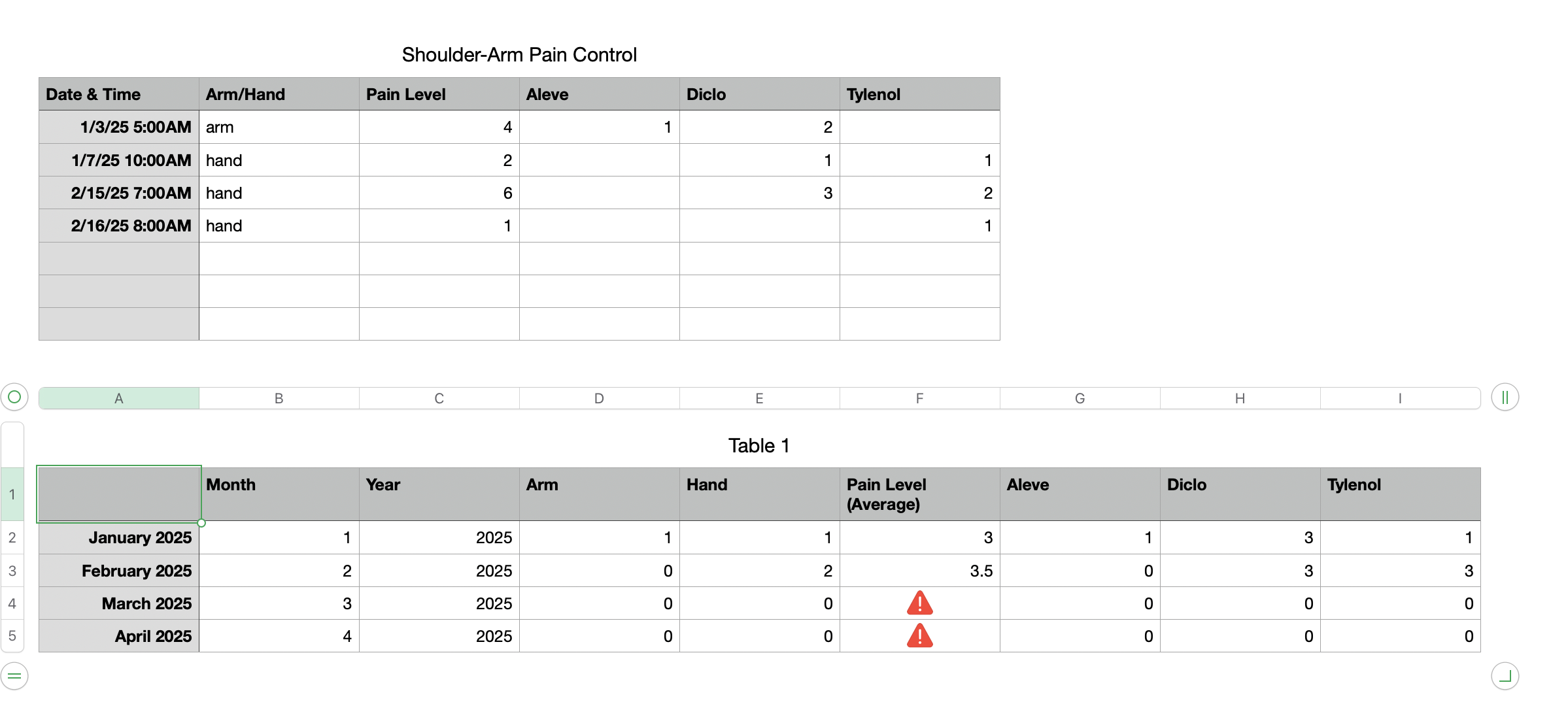
Here is an old-school SUMIFS version:
Formulas in the lower table:
B2 =MONTH(A)
C2 =YEAR(A)
D2 =COUNTIFS('Shoulder-Arm Pain Control'::B,"arm",'Shoulder-Arm Pain Control'::$A,">="&DATE($C,$B,1),'Shoulder-Arm Pain Control'::$A,"<="&EOMONTH(DATE($C,$B,1),0))
E2 = copy/paste the formula from D2 into E2 and change "arm" to "hand"
F2 =AVERAGEIFS('Shoulder-Arm Pain Control'::C,'Shoulder-Arm Pain Control'::$A,">="&DATE($C,$B,1),'Shoulder-Arm Pain Control'::$A,"<="&EOMONTH(DATE($C,$B,1),0))
Fiull right with the formula from F2 into G2 and change AVERAGEIFS to SUMIFS so it is
=SUMIFS('Shoulder-Arm Pain Control'::D,'Shoulder-Arm Pain Control'::$A,">="&DATE($C,$B,1),'Shoulder-Arm Pain Control'::$A,"<="&EOMONTH(DATE($C,$B,1),0))
Fill right from G2 to do put the SUMIF formulas into H2 and I2
If you have a version earlier than 14.4, you will have to fill down with all those formulas. With 14.4 they will "spill" down into the rest of the rows.
You can hide the month and year columns.
Error triangles in the average column are from having no data for those months. You can put IFERROR around the formula to turn it into something else or you can put a filter on the table to hide those rows or you can simply not have those rows until there is data for them.