Long data copied to wide data

This is actually far more complicated than a simple transpose, since your rows and columns are not directly related, and you're inserting additional columns between the different question numbers.

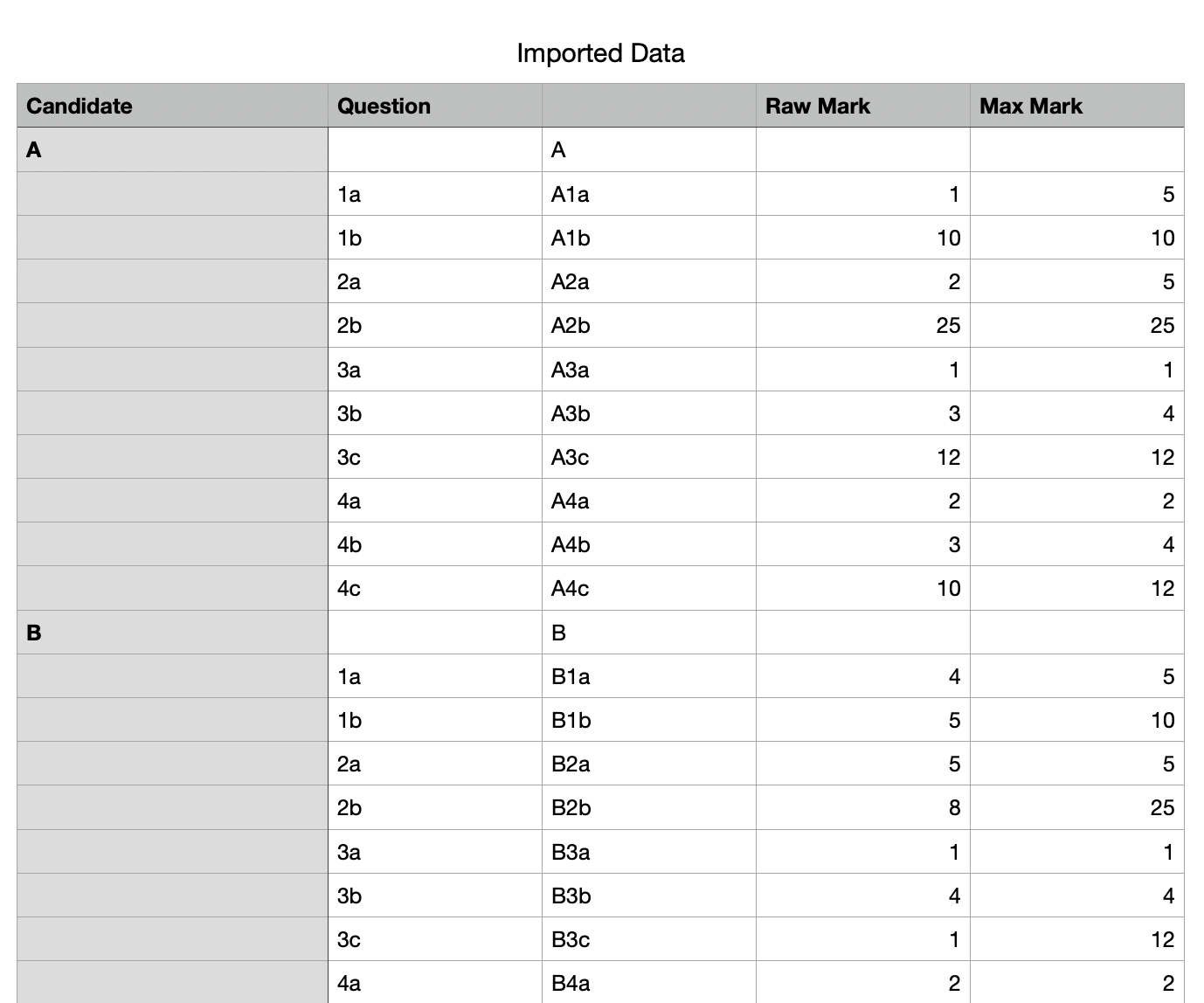
It's also compounded by the fact your source data is not well structured - for example, the candidate name is on its own row, with no score data, and the actual scores have no candidate name attached to them - you have to infer that the scores related to the last-named candidate, and good structured data would never require that leap of faith.

That said, all is not lost.

There are several ways of going about this, but you'll save yourself a LOT of headaches by making one simple change to the source data to provide a key value that incorporates the candidate name and the question.

To do this, I created a new column (C) with the formula in C2 set to:

=IF($A2="",LEFT(C1,1),$A2)&B2

Fill this down the column and you get a cell that combines the candidate name and the question number.

(For aesthetics, you can hide this column since we don't need to see it).

Now we can move on to the summary table.

First, I created a table with just the headers :

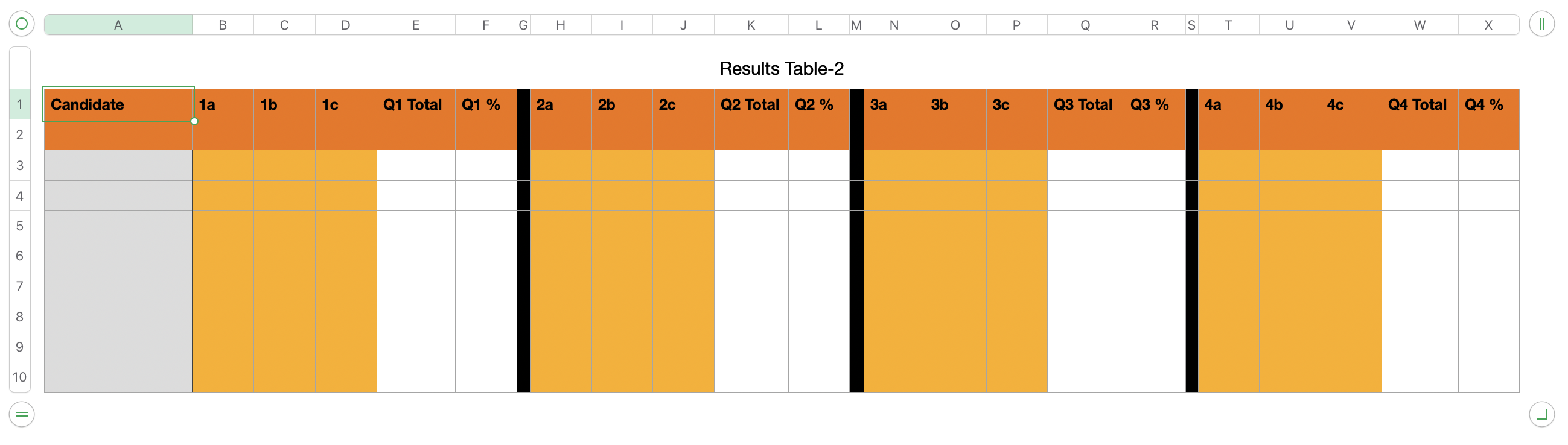
The important thing here is that the headers in row A must match exactly the values from the Questions column in the source data. That's because they're used as the lookup key.

Then, in Row B, set cell B2 to:

=XLOOKUP(B$1,Imported Data:$B,Imported Data:$E,"",0,1)

since the Max Mark values are consistent across all questions we can simply perform a lookup to find any Max Mark value that matches the question number (taken from cell B$1)

You can now enter the calculations for the Question Totals and Question %s (even though we have no values here yet). For example, cell E3 is simply:

=SUM(@ B : D)

to add the values in columns B through D in this row.

This formula can be filled down the column, and copied across to the other Totals columns.

Similarly, you can enter the formulas to calculate the percentages since you now have the max scores and the total for this candidate (yes, the candidate scores are still zero, but we're almost there...)

Right now your table should be looking like this:

now comes the fun part. We need to enter the candidate names and we need to extract their scores.

First, I'll enter the formulas to extract the scores. Set cell B3 to:

=XLOOKUP($A3&B$1,Imported Data::$C,Imported Data::$D,"",0)

This does several things.

First, it combines the cells $A3 and B$1 (the $s are important here) to concatenate the candidate name (column A) with the current cell question label (Row 1). Right now the candidate name is empty, but that's OK.

XLOOKUP() takes that value and looks up a matching value in column C of the Imported Data table - If you recall from the early step, this is the one where we combine the candidate name and the question number.

If XLOOKUP() finds a match, it returns the corresponding value from column D of the Imported Data table, which represents this candidates score in that question.

You can fill this formula across the Q1/Q2/Q3 columns, and down all the rows. Since we have no candidates yet their scores will be blank.

Now comes the magic.

Set cell A3 to:

=UNIQUE(Imported Data::A,FALSE,TRUE)

This piece of magic looks to column A of the Imported Data table and extracts a list of unique values.

This will spill down the column, filling in the candidate names as they're found.

The rest of the sheet will pick up the values in column A, perform the relevant lookups, calculate the totals and %ages.

It's also dynamic. Any time a new candidate is added to the imported data sheet, it should update to include them

Oops, one correction.

The formula on the imported table is too simple, and doesn't properly account for candidate names.

instead of:

=IF($A2="",LEFT(C1,1),$A2)&B2

use:

=IF($A2="",LEFT(C1,LEN(C1)−LEN(B1)),$A2)&B2

which properly prepends the name.

Additionally, in retrospect, it may be better to add this column at the end of columns, rather than inserting in the middle. This will make the table easier to update with new data by copy/pasting the data in, without having to jump over the key column.

With that change, my results table now looks like:

Hi Kipp,

Does this help? With the table selected, Menu > Table > Transpose Rows and Columns.

Regards,

Ian.

If each candidate has the exact same list of questions in the exact same order, I think OFFSET can be used to transpose the results from a column into a row for each candidate. But the list of questions in your first screenshot do not match the list in your second so I don't know if this will work or not. For instance, the first table has questions 1a and 1b then 2a but the second table has 1a, 1b and also a 1c. If some have only 1a and 1b while others have 1a, 1b, and 1c, OFFSET is not going to work.

Once that is done, the formulas can be replaced with their values, the table sorted to move all the rows that have candidate names to the top, and the rest of the rows deleted.

Are you using Excel? If so, you might be better off asking in a Microsoft forum.

https://support.microsoft.com/en-us/excel

https://techcommunity.microsoft.com/category/microsoft365/discussions/excelgeneral

It sounds as if what you want to do is make the columns rows and the rows columns. Perhaps this will help:

https://support.microsoft.com/en-us/office/transpose-rotate-data-from-rows-to-columns-or-vice-versa-3419f2e3-beab-4318-aae5-d0f862209744

If you're transferring the data from Excel to Numbers, do the change in the Excel sheet before copying and pasting.