INDIRECT with R1C1 reference error in Numbers

It would help immensely if you showed what you're trying to do, to understand whether INDIRECT() is needed at all.

The reason I say this is because nothing in your post indicates that you need INDIRECT(), since a relative reference would work just as well.

For example, if you have a column of values in column B and set cell C3 to:

=$B2

AND mark the formula to Preserve Column, then this will automatically copy the value from cell $B2.

The Preserve Column flag (as indicated by the $ in front of the column label) means that it will always reference the same column, whereas the row number will 'float' to be one above the current row. As this formula is filled across or down, the $B will stay the same, and the row number will always be one less than the current row.

If you did want to use INDIRECT(), the corresponding formula would be:

=INDIRECT("B"&ROW()−1)

but that's a lot more work.

EDIT: I noticed the original title referred to R1C1-style references. If you're really trying to use them, the format would be:

=INDIRECT("R"&ROW()−1&"C2",0)

where "R" & ROW()-1 results in Rx, where x is one less than the current row number, combined with C2 for the second column (Column B), plus the ',0' flag to tell Numbers to use R1C1 instead of A1-style references.

OFFSET is another possible choice

=OFFSET(@B,-1,0) is the cell in column B one row up from the formula. If you are using a Numbers version prior to 14.4, leave off the @.

Alternatively

=OFFSET(B4,-1,0) is cell B3

> Go to row 2 and "add row below" in order to add another shift. Then IF(A2=A3... becomes A2=A4.

hmm.. I can see that... not consistently, but sometimes the heuristics that Numbers uses to determine how to adjust the sheet when inserting rows does err in this case.

In which case, I'll defer back to your original ask about INDIRECT(), or maybe BadUnit's OFFSET() although I'd incorporate it into my model.

In that case, E2's formula would be:

=IF(OFFSET(E2,0,−4)=OFFSET(E2,1,−4),"",SUMIF(A,A2,D))

or

=IF(INDIRECT("A"& ROW())=INDIRECT("A" & ROW()+1),"",SUMIF(A,A2,D))

Another alternative that may just be simpler all around is a pivot table, which is designed to help categorize and summarize data. In this case it doesn't even matter what the order of the rows are, and you don't need the 'Daily Hours' column since the Pivot table will take care of summing the individual shift times.

To create a pivot table, select any cell in the table and choose Organize -> Create Pivot Table.

Drag the Date field to the Rows section, and add the Shift Hours and Target Hours to the Values. You should get something like this:

Pivot tables don't automatically recalculate, so you're free to amend your source data as much as you like, and when you're ready to summarize, just click the Refresh Data icon near the top of the Inspector.

You can also format and filter the pivot table as you like - for example, you can easily filter out days that had no work (assuming there were any) and get something like:

OK, that's why context matters. I don't see how relative references or INDIRECT() is going to help here.

Instead, I think you need an IF() statement to compare the day of this row to the day of the previous (or next) row. If they are the same then you know you have a second work shift on the same day, so you don't need to add the day's allocation.

I'm thinking something like this where I added some additional columns to help show the idea:

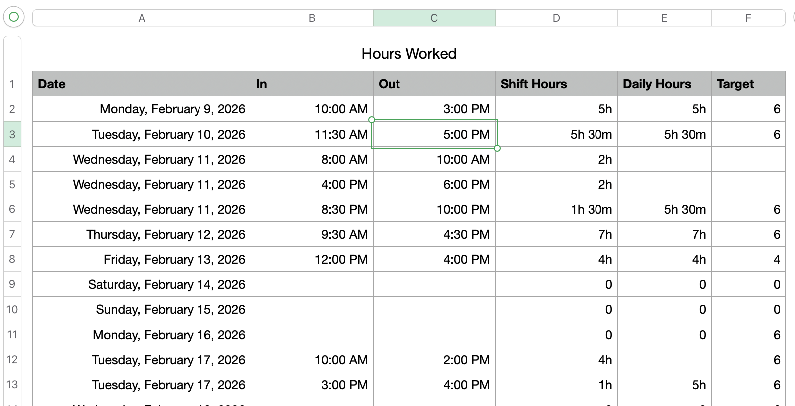
In this table, columns A, B, C, and F match your original template.

(Note that columns B and C are set as Duration cells, which is important when doing time-based calculations.)

Column D is a simple calculation that Subtracts the In time from the Out time to get a number of hours worked on this entry. e.g. cell D2 is simply:

=C2-B2

The first piece of magic comes in cell E2. The formula here is:

=IF(A2=A3,"",SUMIF(A,A2,D))

This says that if the cell A3 (the date of the next shift) is the same as A2 (the date of this shift), then return an empty string. Otherwise, if A3 and A2 are different, add up the values in Column D ("Shift Hours") whose value in column A matches the value in A2.

In other words, this adds up the values of the shifts that match the current date in column A, and only does this for the last shift/row on any given day.

Fill this column down and you'll get the sum of hours worked for each distinct day in column A (you may need to play some games with the last row in the table since it won't have a working day - just create a dummy row with some far-future date, or amend the formula to compensate).

The second piece of magic is column F. For this you need a LOOKUP to find the number of hours that should be worked this day. For that, I did something similar to what I did with the Daily Hours column, and set F2 to:

=IF(A2=A3,"",XLOOKUP(DAYNAME(A2),Target Hours::A,Target Hours::B,0,0,1))

This says that IF the date of this row matches the date in the next row then return an empty string (nothing to do here), otherwise, perform an XLOOKUP where it takes the DAYNAME() of the value in cell A2 and looks that value up in column A of the 'Target Hours' table. For any match, return the corresponding value from column B in the Target Hours table.

This will fill in the expected number of hours based on the DAYNAME() of the date in column A, as long as the next row in the table has a different date. Thus surpassing the value showing multiple times for multiple shifts in the same day.

From here it should be easy to add another column that compares the Daily Hours with the Target hours and flag any days that are over/under, but that's a separate project :)