Highlighting the cell in one column depending on presence or absence of content in another cell the same row .

Conditional highlighting rules compare the value in the cell to be highlighted with another value. The other value can be written into the rule, or can be contained in a different cell.

The usual means of highlighting where the contents of the trigger cell and the cell to be highlighted is to add a third auxiliary cell whose content can be controlled by a formula using the content or state of the tigger cell to produce a value that can be compared with the value in the cell to be highlighted.

Example: The cells in column A are to be highlighted depending on the filled or unfilled state of the cells in column C. The cells on the same row of column G are the auxiliary cells whose value is controlled by the state of the cells in column C, and whose contained value is compared with the value in column A to determine if highlighting is to be applied to that cell.

Note that the formula shown fails to satisfy the rule (see below) when it returns a zero from the empty cell A10, which the highlighting rule (shown below) does not accept as a match for 'empty'. does not accept that zero as a match for 'empty'. This will be an issue only if you have rows where the cell to be highlighted is empty and the trigger cell is filled.

Regards,

Barry

If you want to do it without any extra column(s), it depends on how tricky you want to be and how much you expect out of it. At least I think you can do it. I came up with this idea just now so it requires some testing.

If you want to highlight cells in column B based on whether column C is empty or populated, and if you can guarantee that no value in column B will ever start with the same character(s) as its corresponding cell in column C, you can do a rudimentary highlighting based on C being populated or empty.

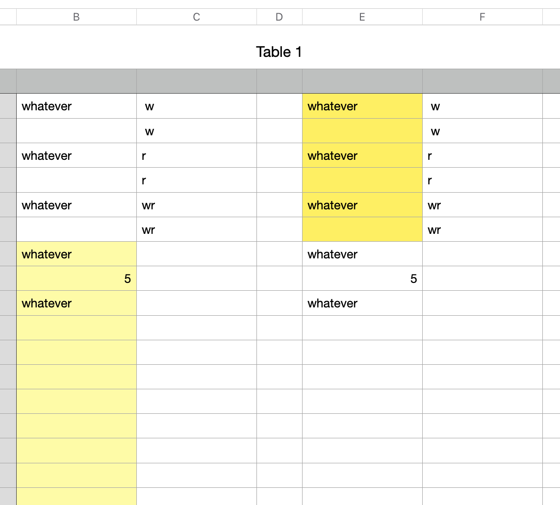
Notice that nothing in column B begins with the letters in the corresponding cell of column C. C2 has a space before the w. If you can pad the values in column B or C with a leading space or other character (that the other column will never have), that should be sufficient.

To create the custom format for column B

1. Select all cells in B (other than header and footer)
2. Create a custom highlight of "Text starts with"
3. Instead of typing in a value, click the green oval on the right side of the text box and then click on cell C2 in the table.
4. Choose the yellow fill (or whatever format you want)

To create the opposite format for column E,

1. Select the cells in column E
2. Format them as yellow background
3. Create a custom format of "text starts with" but click on cell F2 this time
4. Choose a custom fill that will look like the other cells in the table, black text on a white background

If you don't like a leading space, you could try a trailing space and use "text ends with" as the format.

Good luck. I hope it works as intended.