Conditional Formatting Color column select

EDIT: Not really solved. I misinterpreted your post. I was thinking you had this popup in cells A1:A20. The infor below only applies to the cell with the popup.

Conditional highlighting. You will find the button for it in the "Cell" tab in the sidebar on the right side of the window. You would set up 15 rules. Each would be "text is" and you would type in the word and choose a format or create a custom format for that word. Only 15 rules are allowed.

I realized too late my post did not answer your question. Conditional Highlighting in Numbers was designed to highlight a cell based on its content. You are asking to highlight cells based on the content of a different cell. That's an entirely different animal but it can be simulated. It is a lot more complicated. For 15 rules, I think the best option would be to create a second table for the highlighting and slide it underneath your table so the highlighting shines through and appears to be in your table.

There are other posts on how to set it all up. Basically it is this:

1. Create a new table the same size as the one you have, or at least the one column you want highlighted.
2. Cells A1 though A20 get the formula =Table 1::A$1 (assuming your other table is Table 1)
3. Create the highlighting rules in this table. cells A1:A20 will be "text is" and you will type in Apple, Orange, etc. to create all 15 rules.
4. Select all the cells then change the text opacity to zero. (Select the cells, go to the Text tab in the formatting sidebar on the right, click the color wheel for the text color, drag the opacity slider to 0.)
5. Put this table on top of your other one and line it all up.
6. With it selected use Arrange/Send to Back to put it behind your table.
7. You can get back to it if you need to by sliding the top table over a little to uncover some of it so you can select it.

Here is an example of the multiple table method.

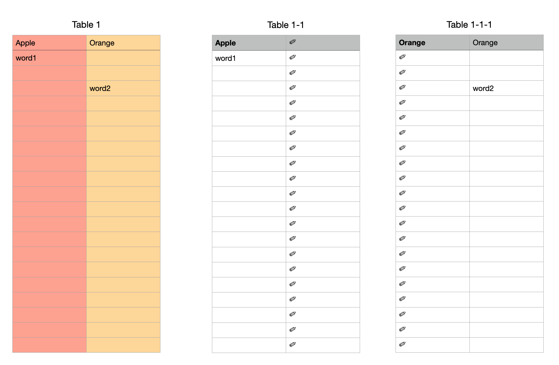
Table 1 row A has your popup.

The rest of Table 1 has a few words typed into it but most is blank.

Make Table 1-1

I typed in the word Apple in cell A1

A2 =IF(Table 1::A$1=$A$1,Table 1::A2,CHAR(10000))&""

Fill across and down to complete the columns. Copy/Paste it to cell B1

I use CHAR(10000) because it is rarely used as far as I can tell. You can use a different character or use several characters to make it even more rare.

The next table is cookie-cutter.

Duplicate Table 1-1 to make Table 1-1-1

Change the word in cell A1

Create the highlighting rules in Table 1.

Select cells A2:B21

Make a rule "text is" and choose cell A2 from Table 1-1

Make a second rule of "text is" and choose cell A2 from Table 1-1-1

In the end you can cut/paste the highlighting tables to a different sheet or you could have put them in a different sheet to begin with.

Hi John,

I am confused about your overall aim. If you choose Apple from the Pop-Up menu in cell A1, do you want all cells in column A to show a green fill, or only those rows in column A that contain the text "Apple" to show a green fill?

Please post a screen shot showing the contents of the cells in column A.

More Information may lead to a solution.

Regards,

Ian.

Yes, conditional highlighting is limited to comparing the value in the cell to something else. If you want to do something other than that it takes some work, if it is possible at all. There are other ways to accomplish conditional highlighting that simulate conditioning off another cell. Maybe one day Apple will improve it to allow conditioning solely off another cell. Here are other workarounds:

If it is a single rule to be applied (highlighting is either on or off), it can be done with one extra column and some trickery. But not with multiple rules. This doesn't apply to your case so I'll not go into it too deeply. The gist of it is the cells in the extra column will either have a null string "" or a character no one ever uses (like CHAR(10000)) and the highlighting rule is "text ends with".

If it is a small number of column of cells you wish to conditional highlight and/or a small number of rules, you can add extra columns to your table, one per highlighting rule. In those extra columns are formulas that fill in the cells based on the value in the "other cell". So, if you picked "Apple" in your popup, all cells in column C would get filled in with whatever was in column A (C2=A2, C3=A3, etc. via an IF statement). If you pick "Orange", all cells in column D get filled in instead. The conditional highlight in column A would be "if text is column C then red background", "if text is column D then orange background", and so on. You hide the extra columns after it is all set up. This is a workable (though not ideal) solution for a single column or a few columns with few rules.

A way I find better than the extra columns is to use extra tables. Instead of putting extra columns in your table, make a new table of the same size, one table per rule. Each cell in one of these tables will have an IF formula just like the columns described above, bringing over the value from its corresponding cell in your main table if it is the rule to be applied. Once you have done one, the others are pretty much cookie cutter. Then set up your highlighting rules. All these extra tables can be on (or cut/pasted to) to a separate sheet away from everything else.

Yeah, its just that you cant do stuff like that in number. Just use Excel and it'll work fine.

All in all it isn't all that much more to do than how you would normally do a conditional format but it is clunky for sure.