You can make a difference in the Apple Support Community!

When you sign up with your Apple Account, you can provide valuable feedback to other community members by upvoting helpful replies and User Tips.

Looks like no one’s replied in a while. To start the conversation again, simply ask a new question.

Numbers 6.2 Conditional Highlighting

I want to use conditional highlighting to highlight a row if a checkbox is checked. Is there a way to highlight a row using an IF formula? For example, using something like IF(F2=TRUE), then cells A2-E2 are highlighted green. This appears doable in Excel, but I can't seem to find how to do it in Numbers.

Posted on Nov 11, 2019 5:57 PM

Reply
Question marked as Top-ranking reply

Posted on Nov 11, 2019 7:06 PM

It's not that easy to conditional highlight a whole row in Numbers (though it would be easy to highlight just the cell with the checkbox). To do the whole row you would need extra columns or a "shadow" table. Using extra columns you could do something like this.


The rule was entered by selecting A2:F8, then choosing Conditional Highlighting, adding a rule and clicking the address token before clicking cell G2 to get the rule as shown in the screenshot.


The formula in G2, filled down an right in the extra columns, is:


=IF($F2,A2,"X")


Substitute ; for , if your region uses , as a decimal separator.


This simply duplicates the value in the appropriate column on the left if F2 is TRUE (checked). Otherwise it inserts an X or some other value you are unlikely to have in the original columns. Then the Conditional Highlighting rule checks to see whether the value in the "original" cell in the leftmost columns is equal to the value in the corresponding cell in the additional columns, which can be hidden after you've got the Conditional Highlighting to work.


Because this involves additional columns I don't usually do this, but instead make the row stand out in other ways. Often using Categories (Organize > Add Category) is an effective way to identify which rows are "complete".


SG


Similar questions

4 replies
Question marked as Top-ranking reply

Nov 11, 2019 7:06 PM in response to Slaunman

It's not that easy to conditional highlight a whole row in Numbers (though it would be easy to highlight just the cell with the checkbox). To do the whole row you would need extra columns or a "shadow" table. Using extra columns you could do something like this.


The rule was entered by selecting A2:F8, then choosing Conditional Highlighting, adding a rule and clicking the address token before clicking cell G2 to get the rule as shown in the screenshot.


The formula in G2, filled down an right in the extra columns, is:


=IF($F2,A2,"X")


Substitute ; for , if your region uses , as a decimal separator.


This simply duplicates the value in the appropriate column on the left if F2 is TRUE (checked). Otherwise it inserts an X or some other value you are unlikely to have in the original columns. Then the Conditional Highlighting rule checks to see whether the value in the "original" cell in the leftmost columns is equal to the value in the corresponding cell in the additional columns, which can be hidden after you've got the Conditional Highlighting to work.


Because this involves additional columns I don't usually do this, but instead make the row stand out in other ways. Often using Categories (Organize > Add Category) is an effective way to identify which rows are "complete".


SG


Nov 11, 2019 7:14 PM in response to Slaunman

Hi Slaunman,


To add Conditional Highlighting to a whole row, you can use a helper table.

Duplicate your data table (Table 1 in this screen shot) to produce Table 1-1

Formula in cell A2 of Table 1-1 =IF(Table 1::$F2,Table 1::A2,"")

Fill down and right.

Conditional Highlighting in Table 1. Select all the cells where you want Conditional Highlighting.


That rule will automatically adjust in all the selected cells in Table 1.

You can move (Cut and Paste) Table 1-1 to another sheet to "hide" it.


Regards,

Ian.


Edit: Great minds think alike, SG!

Nov 11, 2019 7:14 PM in response to Slaunman

Hi Slaunman,


Conditional highlighting in Numbers does not work well for highlighting entire rows. It can be done with a second table behind the first.

My first table looks like you would expect. The second table is as wide as the first but contains only 1 column.

The text in each cell is "TRUE" with the font color white.

You can see the highlighting rules above. when the checkbox in Table 1 is TRUE it matches the text in the cell and the highlight occurs.


quinn

Nov 12, 2019 7:25 AM in response to SGIII

Thank you all so much for your quick replies and amazing help.


SG, I went with your suggestion, because the tables I am working with are regularly having rows added to them as information needing to be tracked increases - I can easily hide the "shadow" columns, and they will carry the formulas as new rows are added. Getting the checkbox cell to highlight was the easy part, it was the IF formula I was struggling with.


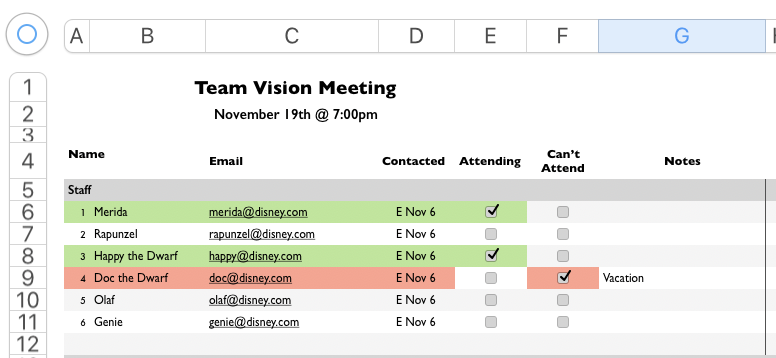
One of my tables is tracking attendance to a meeting ... is there a way to "multi-level" the formula? By that I mean, i have 2 checkboxes, one for attending, one for not attending. I've got it working now to highlight the row green if the attending box is checked, but is it possible to have it highlight red if the not attending box is checked? (Nothing like making it complicated, right? LOL)


When I have more time to explore, I'm going to look into your Categories suggestion as well.


You know, it would be awesome if Apple would add this kind of function to the conditional highlighting toolbox in their next update, just a simple place to put in IF conditions - most everything with Mac is so intuitive, i wonder sometimes how they seem to occasionally miss something that (to me) seems basic.


Thanks again!


Slaunman

Numbers 6.2 Conditional Highlighting

Welcome to Apple Support Community
A forum where Apple customers help each other with their products. Get started with your Apple Account.