How do I grey out unneeded cells in a spreadsheet based on row type?

You are massively over-complicating your spreadsheet by trying to get it to do something it is not designed to do.

While what you ask for sounds simple, it isn't the way Numbers is designed - you cannot push values, formatting, etc. into other cells, and you have to jump through extra hoops to make it work.

I strongly agree with SGIII' suggestion to reformat the data into something more spreadsheet-friendly, maying using filters or pivot tables to summarize the data.

If that's not an option, at least consider a tweak to your layout that will make the whole thing easier.

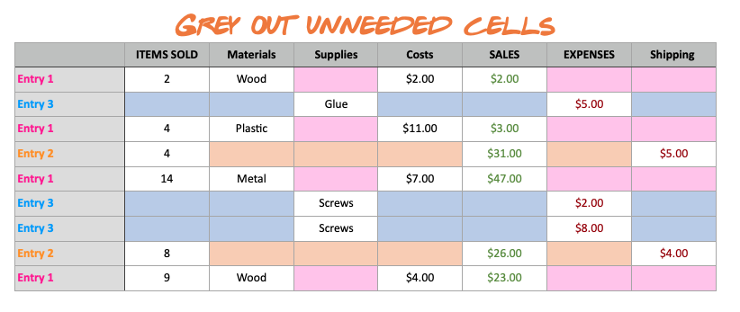
Your current design is keyed off the first column being either SALE or PURCHASE. You're then trying to guide the user to enter values in relevant fields by highlighting (or de-highlighing) the fields in question.

Instead...

What the user cares about (and what's in their head) is four things - a SALE/PURCHASE option, a unit size, price, and a quantity. That is all they should enter and the spreadsheet should do the rest of the work.

For example, based on your sample:

I recreated it with a slight tweak (although your numbers don't make sense, but I'm guessing that's because they're dummy values). I came up with:

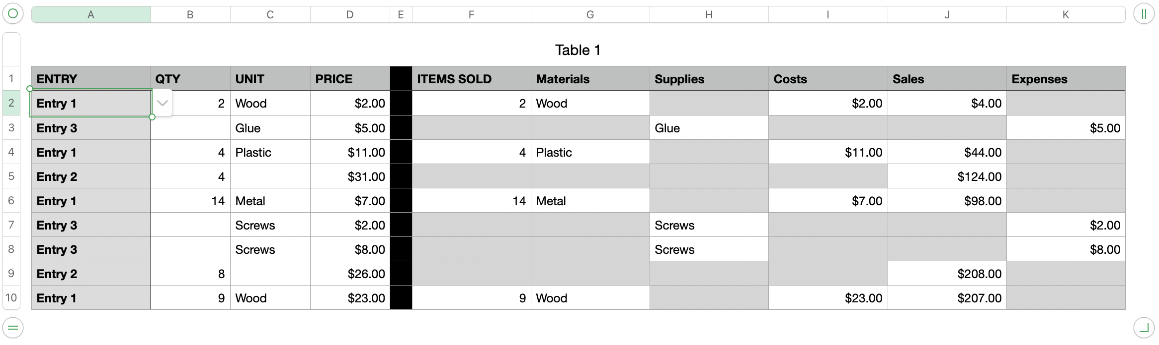
(I skipped Shipping since I couldn't see how that plugged in, but that can be added easily enough once the logic is understood).

The idea here is that the user only enters columns A-D. The rest of the table is filled out automatically based on the values in column A.

There's nothing special about columns A-D, except that column A may be a Pop-up menu with the "Entry' items.

The magic starts in cell E2 (the first 'ITEM SOLD') column. This has a formula:

=IF($A="Entry 1",B)

This says that if the entry in column A is 'Entry 1', then return the value in column B - in other words, copy the Quantity value only if column A says 'Entry 1'.

This will automatically fill in the entire column with corresponding Quantities (or FALSE if column A is not 'Entry 1')

A similar approach is used for the other columns - check $A to and show or hide the corresponding value based on whether it's relevant or not.

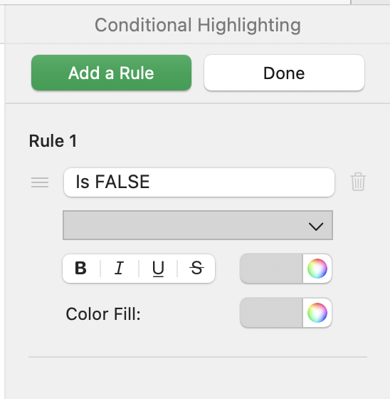
Now all you need to to is add one conditional highlight to the entire table (or, at least columns E-K) that hides the values (based on setting the background and text colors the same):

In this way, column A is used as a trigger to determine whether a value should be shown in the corresponding column or not.

Note that columns E-K could be in the same table, or in a separate table. it's mostly a matter of how you want to visualize your data.

Not a direct answer to your question; I think this could be done with Conditional Highlighting, but it might get complicated.

I recommend you consider entering and keeping your data in a more spreadsheet friendly format, something like this:

You mentioned you have many other columns. That can quickly get cumbersome. The "data in a tabular format" approach can reduce that problem, make it easier to enter data, and also open up possibilities for easy summarization of your data.

For example, with just a few clicks and drags (no formulas!) I produced this:

If you have a date column in the tabular data then you can easily summarize by quarter, month, day of week, etc.

Intro to pivot tables in Numbers on Mac - Apple Support

SG

This will take some time, especially if you have not created highlighting rules before. I think what I am showing below fits the bill but I'm not 100% sure. Each column has its own set of rules. Hopefully you can find an older thread here that goes step-by-step through making rules for a column of cells all at once (vs one cell at a time), creating a rule that compares each cell to a corresponding cell in a different column. I thnk it has been explained in threads for how to highlight an entire row. It is easy to do but kinda tedious to explain.

These rules are all "highlight if the text does not end with the contents of a cell in a different column". I'm using it as a detector for if the other cell is blank or not. If the other cell is blank then the text does end with the contents of the other cell and the highlighting rule does not trigger. If the other cell has something in it, it triggers the highlighting. If you accidentally enter something in two columns that are supposed to be mutually exclusive (like materials and supplies), the highlighting in that row will be wrong.

[Edited by Moderator]

I don't fully follow the "logic" in your second example table, especially rows 5 and 9 where you have neither materials nor supplies, nor do I quite understand your end goal here. An invoice?

However, I would like to take another try at encouraging you to enter your data in more "normalized" tabular format that will make it easier for you to take advantage of the power of spreadsheets. That will also reduce the need for fancy formatting as reminders when entering data.

If you have extra columns this can be somewhat along the lines of:

SG