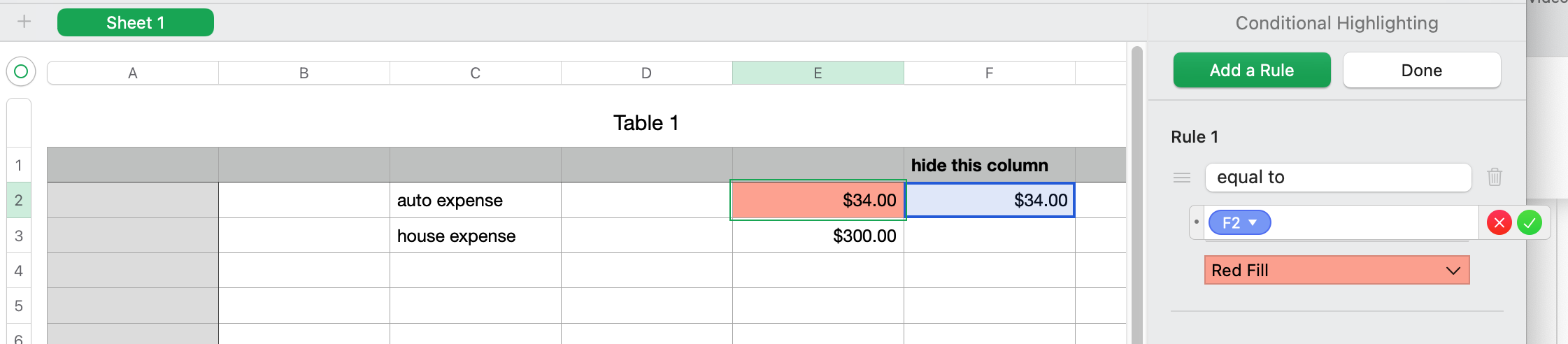
Highlighting is based on the contents of the cell to be highlighted. To highlight cell E2, the rule must have something to do with the value in cell E2. The rule "if C2 is 'auto expense' then highlight cell E2" is not based on the value in cell E2 so it cannot be done. However, you can make a rule like "if cell E2 = cell F2 then highlight cell E2.
What you can do is insert a new column F that has the formula IF(C2="Auto Expense", E2, ""). The highlighting rule in cell E2 would be "if cell E2 is equal to cell F2 then red fill".
For the formula in column F, the usual one is the one given above
=IF(C2="Auto Expense", E2, "")
but I have been inclined recently to use the formula below instead because sometimes "" (null string) is an actual value and it will highlight red when you don't want it to
=IF(C2="Auto Expense", E2, CHAR(10000)).
the chosen character is highly unlikely to ever occur in a spreadsheet.
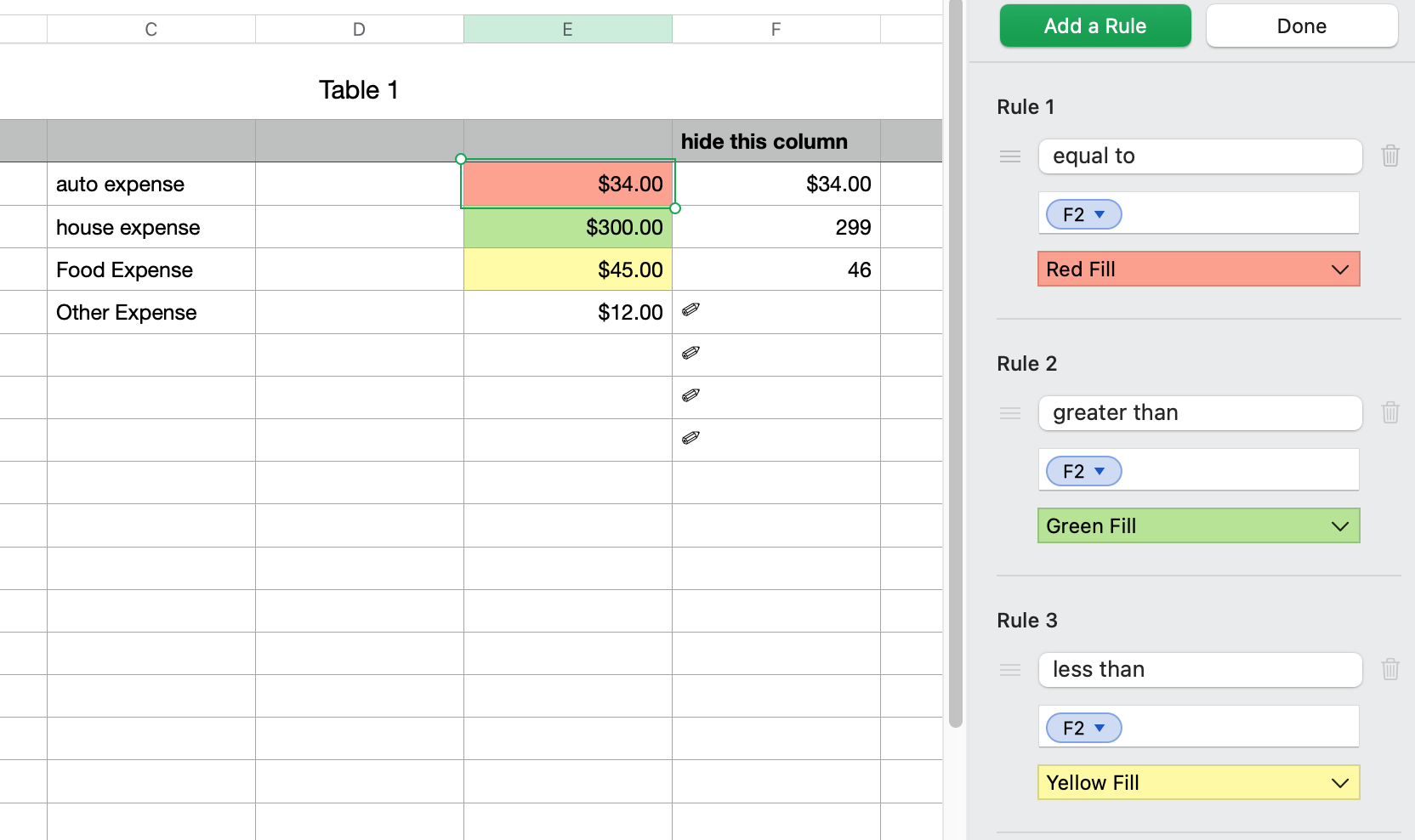
If you want multiple highlighting rules, you can get more clever. The formula below will get you three different possibilities:
=IFS(C2="Auto Expense", E2, C2= "House Expense",E2−1,C2="Food Expense",E2+1,TRUE,CHAR(10000))
If you want more than three rules, it is better to use multiple new columns, each with its own formula
=IF(C2="whatever", E2, CHAR(10000))
and the rules will refer to each of those columns.
"if E2 = F2 then red fill"
"if E2 = G2 then green fill"
"if E2 = H2 then yellow fill"
etc.
Probably more info than you wanted.